대표어
대표어
 학술연구정보서비스(KERIS)
권호기사보기
| 기사명 | 저자명 | 페이지 | 원문 | 기사목차 |
|---|
결과 내 검색
동의어 포함
Title Page
Contents
1. Introduction 13
2. Spatial Regression Models 21
2.1. Simultaneous Autoregressive Model 21
2.2. Conditional Autoregressive Model 23
3. Inference 26
3.1. Classical Inference 26
3.2. Novel Interval Inference 30
3.3. Extending to Inference for Functions of Model Parameters 35
4. Prediction 37
5. Application 39
5.1. Simulation Study 39
5.2. Real Data Analysis 61
5.2.1. COVID-19 in Seoul 61
5.2.2. House Price in Seoul 73
6. Conclusions 83
References 86
요약 91
Figure 1. Approximate population across 925 cities of the United Kingdom in January 2006. 15
Figure 2. Maximum speeds at the major road types (motorway, trunk, primary, secondary, tertiary) in Essex, United Kingdom. 16
Figure 3. Number of the SIDS in North Carolina state during 1974. 17
Figure 4. (a) CPs and (b) ALs of 95% CIs for σ² and β in the SAR and CAR models with p=1 for a 5 × 5 regular lattice. 43
Figure 5. (a) CPs and (b) ALs of 95% CIs for σ² and β in the SAR and CAR models with p=3 for a 5 × 5 regular lattice 45
Figure 6. (a) CPs and (b) ALs of 95% CIs for σ² and β in the SAR and CAR models with p=1 for a 10 × 10 regular lattice. 47
Figure 7. (a) CPs and (b) ALs of 95% CIs for σ² and β in the SAR and CAR models with p=3 for a 10 × 10 regular lattice. 49
Figure 8. (a) MSEs and (b) biases of estimators in the SAR and CAR models with p=1 for a 5 × 5 regular lattice. 51
Figure 9. (a) MSEs and (b) biases of estimators in the SAR and CAR models with p=3 for a 5 × 5 regular lattice. 53
Figure 10. (a) MSEs and (b) biases of estimators in the SAR and CAR models with p=1 for a 10 × 10 regular lattice. 55
Figure 11. (a) MSEs and (b) biases of estimators in the SAR and CAR models with p=3 for a 10 × 10 regular lattice. 57
Figure 12. Boxplots illustrating CPs of the 95% intervals for Y* across a 5×5 regular lattice for (a) p=1 and (b) p=3. 59
Figure 13. Boxplots illustrating CPs of the 95% intervals for Y* across a 10×10 regular lattice for (a) p=1 and (b) p=3. 60
Figure 14. Map for district-level confirmed rates of COVID-19 in Seoul between 02 April 2022 and 08 April 2022. 62
Figure 15. District-level boxplots for the replicated data of the confirmed rates of COVID-19. 66
Figure 16. (a) Map and (b) resulting boxplots of unobserved districts for r=2 in the COVID-19 dataset. 68
Figure 17. (a) Map and (b) resulting boxplots of unobserved districts for r=3 in the COVID-19 dataset. 69
Figure 18. (a) Map and (b) resulting boxplots of unobserved districts for r=4 in the COVID-19 dataset. 70
Figure 19. (a) Map and (b) resulting boxplots of unobserved districts for r=5 in the COVID-19 dataset. 71
Figure 20. (a) Map and (b) resulting boxplots of unobserved districts for r=6 in the COVID-19 dataset. 72
Figure 21. Map for district-level average transaction price per square meter for apartments in Seoul for July 2020. 74
Figure 22. District-level boxplots for the replicated data of the average transaction price per square meter for apartments. 77
Figure 23. (a) Map and (b) resulting boxplots of unobserved districts for r=2 in the house price dataset. 78
Figure 24. (a) Map and (b) resulting boxplots of unobserved districts for r=3 in the house price dataset. 79
Figure 25. (a) Map and (b) resulting boxplots of unobserved districts for r=4 in the house price dataset. 80
Figure 26. (a) Map and (b) resulting boxplots of unobserved districts for r=5 in the house price dataset. 81
Figure 27. (a) Map and (b) resulting boxplots of unobserved districts for r=6 in the house price dataset. 82
본 논문은 면적 데이터(area data)에서 가장 많이 사용하는 두 공간 회귀 모형인 동시자기회귀모형(simultaneous autoregressive model)과조건부자기회귀모형(conditional autoregressive model)의관심있는모수에대한구간추론성능을향상시키는새로운접근방법들을연구하였다.
최대가능도 추정방법은 널리 사용하는 추정방법이지만 모수의 구간을 추정하는데 정확이 아닌 근사적인 결과를 산출하며 피셔정보행렬(Fisher information matrix) 계산과 같은 복잡한 계산과정을 요구한다. 게다가, 면적 단위의 수가 작을 때는 명목수준(nominal level)을 종종 만족하지 않는다는 치명적인 단점이 있다. 빈도주의적 관점에서 이러한 문제를 해결하면서 추론 성능을 향상시키기 위해 우리는 추축량(pivotal quantity)과 몬테카를로 시뮬레이션(Monte Carlo simulation)을 활용한 새로운 접근방법들을 제안하였다. 관심있는 척도(scale) 모수와 회귀(regression) 모수에 대해 추축량을 활용하여 간단하면서 정확한 신뢰구간(confidence interval)을 제공하였으며, 회귀 모수에 대해서는 추가적으로 추축량과 몬테카를로 시뮬레이션을 활용한 방법도 제공하였다. 이 방법은 장애 모수를 적절히 처리하는 방법을 통합한 알고리듬을 도입함으로써 수행하며, 도입된 알고리듬의 매력은 뛰어난 확장성을 가진다는 점이다. 우리는 이러한 확장성의 구체적인 예시로 관측된 데이터의 샘플링 분포(sampling distribution)를 추론하면서 복제 데이터(replicated data)를 생성하는 알고리듬을 소개하였다. 게다가, 관측되지 않은 면적 단위에 대한 예측 문제를 해결하기 위해 예측 알고리듬도 제공하였다.
제안된 접근방법은 시뮬레이션 연구와 실제 데이터 분석에서 타당성이 증명되었다. 시뮬레이션 연구에서는 다양한 세팅을 통해 면적 단위의 수가 작거나 중간인 상황에서 제안된 접근방법이 최대가능도 추정량에 기반한 추론방법보다 우수하다는 것이 증명되었으며, 실제 데이터 분석에서는 제안된 접근방법의 적용가능성이 점검되었다. 결과적으로 제안된 접근방법은 기존의 최대가능도 추정방법과 비교하여 경쟁력을 가진다는 사실을 알 수 있었다.*표시는 필수 입력사항입니다.
| 전화번호 |
|---|
| 기사명 | 저자명 | 페이지 | 원문 | 기사목차 |
|---|
| 번호 | 발행일자 | 권호명 | 제본정보 | 자료실 | 원문 | 신청 페이지 |
|---|
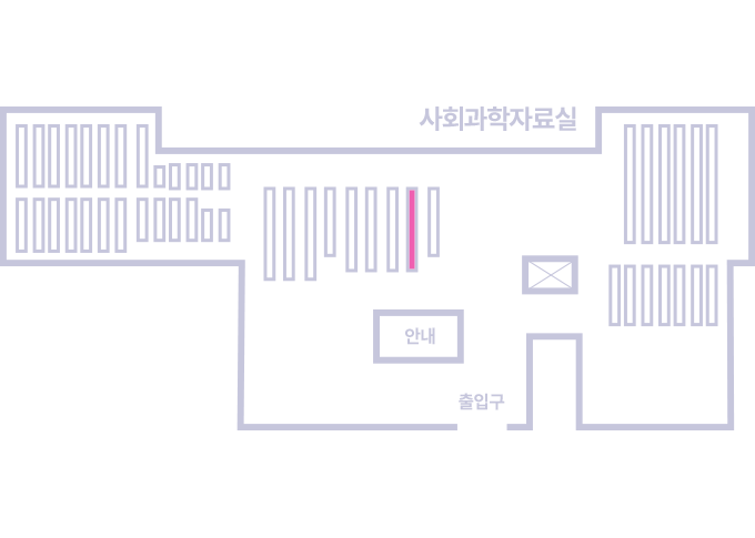
도서위치안내: / 서가번호:
우편복사 목록담기를 완료하였습니다.
*표시는 필수 입력사항입니다.
저장 되었습니다.